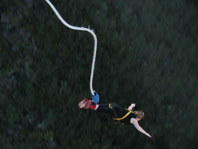
Demonstration: Bungee Jumping

The following second order non-linear differential equation models a bungee jump:

\[m y''(t) + m g + b(y(t)) + \beta y'(t) = 0.\]

Here y(t) denotes the position of the jumper at time t; m is the mass of the jumper, g is the gravitational constant, and \(\beta\) is the damping coefficient due to air resistance.

A bungee cord acts like a spring when stretched, but it has no restoring force when "compressed". The restoring force of the bungee cord b(y) is thus modeled as follows:

\[b(y)=\left\{\begin{array}{cc}k y,&\mbox{ if } y\leq 0\\0, & \mbox{ if } y>0\end{array}\right.,\] with \(k\) being the spring constant of the bungee cord.

The graph below shows the position y(t) and the acceleration \(y''(t)\) of the jumper at time t. The dashed line shows the equilibrium solution, i.e. the position of the jumper at the end of the jump. The natural length of the bungee cord is 100 ft, and the jump starts at a height of 100 ft.

You can change the weight w of the jumper, the damping coefficient \(\beta\), and the spring constant k of the bungee cord.